Fun with Matlab: Calculator

Calculator is a simple number computing device and building it is a complex task. However if we forget about hardwire complexity behind it and shift ourselves to the software technology, making computing device, i.e. calculator is not much difficult. All you need is little bit of logic, mathematics and programming. Being a communication engineer, Matlab is my best programming platform and I love to have some fun with it in free time. I have made two different calculators, one having simple input output and another having numeric keypad and display using Matlab GUI.

As shown in figure above is my “calc.m” which is able to calculate basic operations: add, subtract, multiply and division. To use this calculator, first give inputs and then choose operator and then click to result button. You have to strictly follow these steps: input, choose operator and result, each time you change inputs or operator to get the correct result. To view the source code, click here.

This is “calculator.m” able to calculate basic four mathematical operations. To use this, click CE button at first so that it shows display 0. Now you can start computing like clicking 9, then 5 so that it displays 95 as your first number. Then click operator like +. Then give second number like clicking 5. Now click = button to see the result as 100 in this case. To start next computation always click CE button, otherwise you will get wrong result. To view the source code, click here.

Matlab Work: Electric field pattern of two isotropic sources (same amplitude with phase difference from 0 to 360 degree)

Electric field pattern is the graphical representation of radiation properties of isotropic sources with their governing mathematical equations. Graphical representation is very important aspect for engineering students in order to visualize facts and real time scenarios. The purpose of this simulation in Matlab GUI is to plot the electric field pattern of two isotropic sources placed in x-axis on either side of origin having same amplitude and variable phase difference. The GUI allows us to understand the field pattern at different phase difference ranging from 0^o to 360^o. The isotropic sources are as follows:

Assumption made is that the two isotropic sources are source 1 and source 2. Let their constant electric field E_o=0.5 V/m and distance of separation d=λ/2. So the relative distance between sources expressed in radian becomes d_r=2πd/ λ=2π(λ/2)/ λ= π. So the general electric field expression: E=2E_o cos(d_rcosφ/2) + (δ /2) reduces to

E=cos(π cosφ/2)+ (δ /2)………………………………….(i)

which can be easily plotted in Matlab. Here φ is the phase angle that also varies from 0 to 360 degree (0 to 2π). 

The plot of E field vs φ for phase difference δ=0⁰ is shown as below. I have used a slider in GUI that has range from 0 to 360 degree and it facilitates us to have virtual analysis as like in real time environment.  

The pattern equation for δ=0⁰ from equation (i) is E=cos(π cosφ/2). The patterns are a bidirectional figure of eight with maxima along the y direction, i.e. normal to the arrays.

Similarly the E patterns for different phase values (δ) are as below:

δ=90^o(π/2)

Field equation is E=cos(π cosφ/2)+ (π /4).

 

δ=180^o(π)

Field equation is E=cos(π cosφ/2)+ (π /2). Field pattern is a relatively broad figure of eight with the maximum field in the same direction as the line joining the source (x-axis).

δ=270^o(3π/2)

Field pattern is E=cos(π cosφ/2)+ (3π /4)

The field pattern tool was very helpful during my Antennas and Propagation course of 7^th semester. You can try similar for the field pattern of more than two isotropic sources or simply for two isotropic sources placed in y-axis, provide the knowledge of field equations.

To view source code, click here. 

Matlab Work: Optimum Cluster size, Number of cell and User support

Cellular mobile communication is one of the major branches of wireless communication which gives mobility and service to the user. The main technologies that are currently being used are GSM (Global System for Mobile) and CDMA (Code Division Multiple Access). In Nepal, NTC and Ncell have adopted GSM system, while Sky phone use CDMA technology. Although both GSM and CDMA divide their available frequency band into channels, the main difference between these two technologies is GSM uses certain number of frequency channels in a cell and each user get their own frequency channel, while CDMA uses only one frequency channel in a cell with proper allocation of PN (pseudo-random) code to each user. PN code is a special set of numbers which is mixed with the modulated signal during transmission and transmitted message can be decoded only with the same PN code. 

 

Analysis of GSM system with mathematical model in Matlab is very useful for communication design engineers. My work is to find the optimum cluster size, number of cell required and user support for a GSM system with the help of MATLAB GUI. I put some design equations in this GUI and created simple model as shown below.

A cluster is a group of cell with different set of frequencies. It can only be acceptable numbers like 1,3,4,7,9,12,… so that cluster size 7 means there are only seven different cells in the system that use different frequencies and other cells are only the reused pattern of these cells. By knowing the suitable cluster size one can estimate the channel required and estimate the bandwidth of their system. 

Total number of cell refers simply to the number of towers required, i.e. cost of the system (Generally, one cell requires one tower for communication purpose). If we also know the area of a cell, than we can estimate the terrestrial coverage of the system. User support indicates the total number of users using the system. It helps to calculate percentage penetration.

The input parameters required for this GUI are SNR (i.e. accepted level of signal to nose ratio; SNR=18 means system’s SNR should not be less than 18dB), path loss (depends on the terrain or terrestrial condition like it is free space, village area or urban area; for urban n=4), GOS (measure of ability of user to access the trunked system, if GOS=2%, then out of 100 users trying to access a trunked system, 2 users are blocked and only 98 users can access the trunked system), Total area of cell and Channel per Cell(we have to specify at most channel the system can provide for a cell).

 

Sectoring is the process of splitting a single cell into different sub-cells. I have given the facility of simulating the case of sectoring and type of cell area in this GUI. Sectoring options include (i) no sectoring, (ii) 120^o sectoring and (iii) 60^o sectoring. Similarly types of cell area are differentiated as small, medium and large. Small cells refer to the average area of 1km², Medium cells refer to 5km² and large cells refer to 10km².

 

Let us view the GUI simulation for the inputs and outputs as shown in figure.

Input are SNR=15 dB, path loss n=4, GOS=2%, total area of cell=2500 km², channel per cell=20, no sectoring and medium sized cells. So the cluster size we should use is of 7, i.e. we should use at least seven cell of different sets of frequencies. Using this scheme, we can cover 500 medium cell area and support up to 65500 users

To view source code, click here. 

(Acknowledge: Brajesh Mishra, Lecturer, DoEE,Kathmandu University)

Maxwell’s Equations: Light-An electromagnetic wave

Light, a mysterious thing; people said that it is a ray; physicist said that it is a photon beam, and Faraday said it is an electromagnetic wave. No one believed him, some physicist laughed at him, until Maxwell came with mathematical solution. A different idea, different thought and perception built on the basis of four equations. It was not only the problem solving in advanced mathematics, but changing the concept of people, changing the vision of scientists and physicists; to understand universe, to understand the hidden mystery and to know how god created this world.

 

The understanding of light and wave in terms of Maxwell’s equations is easy and efficient. But if asked, most people outside physics would not be able to identify Maxwell’s equations, nor would they be able to state that they dealt with electricity and magnetism. However, Maxwell’s equations have many very important implications in the life of a modern person, so much so that people use devices that function on the principles in Maxwell’s equations every day without even knowing it.
 

I, being an engineering student can see its use in day to day life. Even in the lectures of Optical fibers, Antennas & wave Propagation, we use them to find Electric and Magnetic fields of radiation pattern of antennas in different coordinate systems. Many of us used to get bored solving the equations because of calculation complexity and problem in interchanging coordinate system. Obviously, they are challenging but I respect these four equations and never forget as long as I live.
 

1. Gauss’ Law for electric fields: ∇.D=ρ

The electric field tends to point away from positive charges and towards negative charges. More technically, it relates the electric flux through any hypothetical closed "Gaussian surface" to the electric charge within the surface.

The divergence of the outgoing electric field over an area enclosing a volume equals the total charge inside, in appropriate units.
 

 2. The corresponding formula for magnetic fields: ∇.B=0

There are no "magnetic charges" (also called magnetic monopoles), analogous to electric charges. Instead the magnetic field is generated by a configuration called a dipole, which has no magnetic charge but resembles a positive and negative charge inseparably bound together. The total magnetic flux through any Gaussian surface is zero, or that the magnetic field is a solenoidal vector field.

No magnetic charge exists: no “monopoles”.
 

3. Faraday’s Law of Electro-Magnetic Induction: ∇×E= - ∂B/∂t

How a changing magnetic field can create ("induce") an electric field. This aspect of electromagnetic induction is the operating principle behind many electric generators: A bar magnet is rotated to create a changing magnetic field, which in turn generates an electric field in a nearby wire.

The first term is curl of Electric field, usually a wire, and gives the total voltage change around the circuit, which is generated by a time varying magnetic field threading through the circuit.
 

4. Ampere’s Law plus Maxwell’s displacement current: ∇×H=J+ ∂D/∂t

Magnetic fields can be generated in two ways: by electrical current (this was the original "Ampere's law") and by changing electric fields (this was "Maxwell's correction"). Maxwell's correction to Ampere's law is particularly important: It means that a changing magnetic field creates an electric field, and a changing electric field creates a magnetic field. Therefore, these equations allow self-sustaining "electromagnetic waves" to travel through empty space.

Total magnetic force around a circuit in terms of the current through the circuit, plus any varying electric field through the circuit (that’s the “displacement current”).
 

Maxwell’s above equations describe the electric and magnetic fields arising from varying distributions of electric charges and currents, and how those fields change in time.  The equations were the mathematical distillation of decades of experimental observations of the electric and magnetic effects of charges and currents. Maxwell’s own contribution is just the last term of the last equation but realizing the necessity of that term had dramatic consequences. It made evident for the first time that varying electric and magnetic fields could feed off each other; these fields could propagate indefinitely through space, far from the varying charges and currents where they originated.  Previously the fields had been envisioned as tethered to the charges and currents giving rise to them. Maxwell’s new term (he called it the displacement current) freed them to move through space in a self-sustaining fashion, and even predicted their velocity it was the velocity of light!  
 

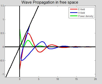
Maxwell solved these equations and the important two equations came, this gave the idea about light being a wave. Physicists started talking about wave nature of light and in the history of physics; it climbed one more step in a long endless journey.These were space and time dependence of electric and magnetic field. It was clear from these equations that the free space propagation of wave, which was variation of electric(E) and magnetic(B) field can only occurs at a particular speed c=2.99×10⁸ (m/s), which was the speed of light(c). In free space, wave propagates at the speed of light. Faraday was true! Maxwell had proven Faraday! Light is an electromagnetic wave.
 

The concept for the understanding of light helped Einstein for the discovery of his world famous equation: E=mc². This equation is simply says mass is convertible to energy and the energy is mass times the square of velocity of light. The speed of light is 3×10⁸ m/s, its square is 9×10¹⁶, which is very large. If a small amount of mass is converted into energy than large energy can be created. One thing we have to know is how to disintegrate mass? Scientists of today know it and they have made Hydrogen and Atom bombs using these principles.
 

We human have come so far from the beginning and we have achieved so much. The application of Maxwell’s equations is in various areas. But there are also lots to explore. I suggest readers to use them, try to solve in your own way and luckily you may get different results, may be that would be helpful for understanding our universe more clearly, that may change the perception of people and you may get Nobel Prize.

(This article was published in Annual magazine of department of Electrical and Electronics, encipher-2010)

First day of blogging

Hello everyone, My name is Sudip Shrestha studying electrical and electronics (communication) engineering in Kathmandu University. I want to share my experience, technology, knowledge, etc in this blog.