Saturday, December 17, 2011

Visualization of Electromagnetic wave in MATLAB

Wave is imaginary and mysterious thing to us. Many of them are invisible and we even don’t know their presence, but they exist. The wave coming out from mobile, wave captured by television, FM waves, x-ray waves, etc are common example of waves we encounter in our daily life. Among these all, light, source of energy of our entire planet comes to earth in the form of wave. Waves are actually disturbance, some sort of vibration or oscillation travelling through space and time. Waves in most of the case contain some form of energy and they are responsible for transfer of energy. Technically, these waves are certain form of electric and magnetic fields. So these waves are commonly known as electromagnetic waves. 

In the virtual world of electromagnetism, waves travel amazingly making different function with space and time. The best way to represent their travelling in forward backward direction with space and time is by using sine or cosine function and represent their decay with space and time is by using exponential function.  These waves seem amazing when we actually see them travelling in space. I present here electromagnetic wave plotted in MATLAB.

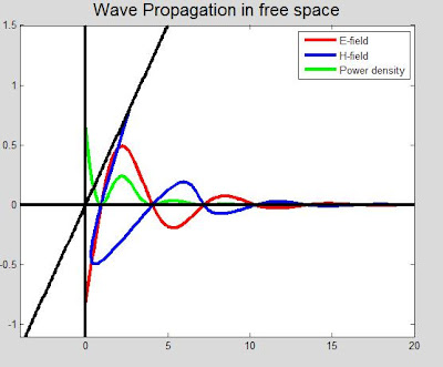
Figure1: Electromagnetic wave in free space

The plot above is a snapshot of traveling electromagnetic wave in free space. The wave is traveling forward along with horizontal black line. The vertical black line and the tilted black line acts as a reference point and considered to be the origin of the wave. Electrical field waves and magnetic field waves are shown in red and blue colors respectively. The power of the wave is actually power density or poynting vector, is shown in green color. 

From the electromagnetic theory, electrical and magnetic fields can be expressed as function of space (z) and time (t) as:


Where, α = attenuation factor of wave.
            β = 2 π/ λ = phase factor of wave
            ω = angular frequency of wave.
            λ = wavelength of wave.
            φ = phase difference between electric and magnetic field. 

The power or the energy carried by these waves is power density (S) given as

S=E×H…………………………..(iii)

Inserting all these equations in MATLAB, my attempt is to make simple GUI which is shown below.

 
Figure 2: Electromagnetic wave visualization tool
 
It is electromagnetic wave visualization tool that I developed in MATLAB. It can plot electromagnetic wave in different parametric condition. “Choose medium” box has three options: ‘Free Space’, ‘Lossless medium’ and ‘Lossy medium’ that plays movie of the electromagnetic waves in those conditions. Similarly, I have made other boxes for different parametric change (You can explore them in GUI figure file). The snapshot of ‘Free space’ is shown in figure 1. Snapshot for other medium are shown in figure 3 and figure 4.


Figure 3: Electromagnetic wave in lossless medium

 
Figure 4: Electromagnetic wave in lossy medium

The electromagnetic wave is simulated in MATLAB is by using ‘movie’ command. This command snaps the different frames first and then plays them in figure window of MATLAB. A small piece of code may be useful to understand the working of plot of electromagnetic wave and ‘movie’ command. 

framemax=20;
M=moviein(framemax);
for z=1:framemax
    E = exp(-t.*a).*cos(w.*t-2*pi*z/framemax); % a = alpha, w = omega
    H = exp(-t.*a).*cos(w.*t-2*pi*z/framemax+phi);
    S = E.*H;
    % plot command
M(z) = getframe(gcf);
end
movie(M)

I have used 20 frames for the simulation. For each frame, it snaps different space value (z) with different sets of time value (t). 

Sunday, August 21, 2011

Guide: How to Install Nagios3 in Ubuntu?


These commands below installs Nagios (Version 3.2.0). Follow these steps carefully.
1.You must work with administrative privilege. So your terminal must be in 'root'. 
Open terminal. If it is not in 'root', type the following command to change it into root:
	$ su
	Password: 
Enter password of root and notice the notation '$' changed to '#'. 
Type 'cd' and your terminal directory looks as shown below: 
	#cd
	root@ubuntu~desktop:/#	
2.Update your Ubuntu.
	apt-get update  
After update, your terminal looks as below:
3.If you have already tried to installed Nagios, then remove it completely by following command:
(optional)
	apt-get remove -purge nagios-common nagios3
4.Install Nagios3
	apt-get install -y nagios3 
During installatiocn, it requires Nagios password. Enter Nagios password.
 
5.Verify the configuration file.
	nagios3 -v /etc/nagios3/nagios.cfg 
After verification, there shouldn't be any errors and warnings. It looks like as follows:
6.Restart Nagios3
	/etc/init.d/nagios3 restart
7.Open any browser and type following in the address bar.
 	http://localhost/nagios3/
 It requires authentication. 
 
        User Name : nagiosadmin
	Password : <default you have set in step 4>
Now you have installed Nagios3. Your Nagios3 in browser is as follows: 
NagiOs is installed, enjoy!!!. 
8.You can change your Nagios3 password by following command (optional)
	htpasswd -c /etc/nagios3/htpasswd.users nagiosadmin

Saturday, June 18, 2011

A new step to JAVA: Baghchal

Baghchal is a Nepali board game, traditionally played in drawn lines on tables with the help of stones. Four big stones used to be "Bagh" and 20 small stones used to be "Bakhra". With the advancement in technology, Baghchal is now available in software. People are now able to play it in their PCs, Laptops. 

As i introduced Baghchal, we may think that i have something to do with it. Yes it has; I have made Baghchal in JAVA. My GUI of Baghchal is shown in figure below.


There are four tigers(baghs) in four corner of Baghchal board. Twenty goats(bakhra) are outside of the board. We can see two messages "Its goat turn" and "Its tiger turn", which are activated and faded according to the turn. If tiger wins the match "Tiger won!!!" will be activated, and if goat wins the match "Goat won!!!" will be activated.

Tiger wins the match if tiger eats at least five goats. The tiger winning situation is as shown in figure below. You can notice that the "Tiger won!!!" message is activated. 


Goat wins the game if goats are able to block all possible path of tigers. It is like locking all four tigers in a cage. Goad winning situation is shown in figure below. You can notice that the "Goat won!!!" message is activated.


Interested can download my game and try at once, click here.
How to play: Instructions (you can find this in README.txt file of baghchel.rar as well)
============================================================
    * place "baghchal" image folder to your "c:\" drive of computer
    * run Baghchal.jar
  
    * to play game press "r" key from keyboard. (r=restart game).
    * use arrow keys (top,down,right,left) for selection
    * use space to place/move object.
        * to palce goat:      select empty location using selection arrow keys
                      and press "space".
        * to move goat/tiger: select goat/tiger to move using selection arrow
                      key. select empty location usign arrow keyand
                      then press "space".
============================================================

Friday, June 10, 2011

Simple block game: Java work

Mr Sulabh Bista wrote an article about different programming languages in SEEE magazine, Encipher-2010. The title of his article "Learn language for life" was an inspiration for me. He suggested four important languages: Phython, PHP, MATLAB, JAVA. I knew MATLAB and i decided to learn JAVA. From then, it has been about 8-9 months and now I am in the level of making simple GUI games (I had made snake and ladder, published earlier in this blog). I also can't help thanking Mr Pranav Nandan for his kind support during my initial learning days. 

Taking about this block game, it is a simple single player game, you have to put all red blocks in brown square to win. The GUI in "stage 1" looks like as shown in figure below:

figure: sample GUI of stage 1

Blue areas are restricted, objects can not go there. To move red object, user has to push it by blue object. User can not push red object if two or more blocks are in same line or there is blue area after red object. To load different stages, press different keys: 1,2,3,4,5,6,7,8,9,0,-,+ (There are all together 12 stages). To move blue object, press: w = up, a = left, s = down and d = right. You can win if you could place all red objects in brown square.

To play game, download "blockgam.rar" file from here
(Warning: Please carefully read "read it.txt" , don't forget to place image folder "blockgam" in C:\ drive of your computer). Please comment down if you have any problems and suggestions about this game.

Tuesday, May 31, 2011

Simple arduino project: Push-button Counter and Calculator

As a hobby project, i decided to build a calculator. Inputs should be given from keypad and outputs should be displayed in two 7 segment displays. In the first stage i had to make two 7 segments work simultaneously. Best solution was to use the concept of time sharing and i did so, each segments turning "on" and "off" in every 5 ms complementary. Then i added a push button in the circuit so that it counted from 0 to 99 and back to 0. 
 
figure: push-button circuit.

In every pulse of push button, value of count increases by 1. When value of count becomes 99, arrival of one pulse reset it to 00. People are suggested to watch this video for the detail of what is happening.  
 
video: pushbutton counter

After push-button, calculator was not so far. I added three more push-buttons. I assigned first push-button to take input of first number, second push-button to take input of second number, third push-button for operation selection and fourth push-button for output or result display. Operation selection logic of third push-button is as follows:
                00 = addition;         01 = subtraction;         02 = multiplication;      03 = division
Please watch what is happening in the circuit.

video: demonstration of calculator

This calculator is able to perform addition, subtraction, multiplication and division of two digit decimal number. Input at the push-button must be given sequentially (i.e. 0-1-2-3-...-99 and back to 0). During the arithmetic operation overflow can occur; so it displays only first two LSB's. Circuit diagrams are as shown below. 
figure: Circuit connection in breadboard and arduino

 
figure: pin configuration of connection in breadboard and arduino

Interested can view the source code, click here.

Friday, May 27, 2011

Robotic Arm Control using Image Processing in MATLAB

When i was in third year (Kathmandu University, Undergraduate Course, EE) our group choose "Robotic Arm control using Image Processing" as our third year project. It was little bit challenge for us, but we finally did it. The basic idea was to pick up selected colored object(red, green, blue) from the board and drop it to the destination container. So our first task was to distinguished objects i.e. whether it was red, blue or green. We developed an image processing algorithm that distinguished red, blue or green colors from captured image of an object. So we captured image (camera was placed vertically upward) of that object placed in the board and fed that image into computer. Then processing algorithm in MATLAB processes the image to select which one to pick. 

 figure: Project platform
But that was no at all. We had to find the position of object; so we developed another algorithm to find center of any circular object. After finding the center of image, we used matching algorithm that matches the center pixel of required circular image with the coordinate of platform. 

Software and hardware part were done; Now we had to move our arm. We needed electrical/logical computer interface to control the arm of robot. We used parallel port that had to control four motors of robotic arm. Our interface circuit was shown below:
figure: interface circuit
The pins D0, D1, D1, D3 and D4 is from parallel ports. 74368 IC is for parallel port protection and logic inversion. There are two 3 by 8 decoders. Combination two outputs of different decoders with relay switching control the robotic arm. In circuit, Y0 of two decoder is controlling output1 (o/p1) and in similar way, Y1 is controlling o/p2, Y2 is controlling o/p3 and Y4 is controlling o/p4. The table showing input output circuit relation is as below.

D0
D1
D2
D3
D4
Motor\Direction
1
0
0
0
0
1st\right
0
1
0
0
0
1st\left
1
0
0
0
1
2nd\right
0
1
0
0
1
2nd\left
1
0
0
1
0
3rd\right
0
1
0
1
0
3rd\left
1
0
0
1
1
4th\right
0
1
0
1
1
4th\left
1
0
1
0
0
5th\right
0
1
1
0
0
5th\left
table: Logic of circuit diagram

The output D0 to D4 are suitable controlled by parallel port using predefined set of algorithm. So, to pick up any object from the desired location, we should give required logic from D0 to D4 for a predefined time. At a time one motor would move. So there was sequence of processes that would move different motors one after another.

  
figure: Robotic arm of project

We had set our logic in such a way that 'base' motor moves first in the desired line, than combination of 'Elbow' and 'Shoulder' takes arm to the destination. Then gripper grips the object and 'Elbow' and 'Shoulder' takes off the object. Then 'Base' moves to the container, and 'gripper' drops the object in the container. 

We had made this whole process to be controlled in MATLAB GUI. Our GUI looked like as shown below.

figure: GUI of robotic arm control

We was three control schemes, one is 'autonomous control' where we had to insert which color object to pick up and it would automatically pick up that object and drop down in the container. 'Manual control' scheme allowed control of Robotic arm by keyboard keys (keys from 0 to 9). 'Grid Control' was to pick up and drop down the object by giving its coordinates (A1,A2). Here you can watch the video of this control system.
video: Picking Green ball and dropping it in container

The project was a like dream project for me. I really enjoyed doing this, and learned a lot.

Friday, May 20, 2011

First Arduino mini project: counter & random number display

It has been about six months since i haven't done any electronics project. May be i was tired with traditional electronics workshop style. Then i brought Arduino uno with Atmega328 micro processor. During learning phase i worked with display in LED and then in 7-segment. Working with LED gave lots of fun (i worked with pranav, sulav). Then i switched to 7-segment: a counter display and a random number display. The circuit of arduino with 7-segment is as shown below:
figure: 7-segment display from arduino 

Digital pins 12,11,10,9,8,7 and 6 are taken as seven bit output pins. These output pins are connected to 7 segment display pins b,a,f,g,c,d and e respectively. Output is active low, that means output segment is on when LOW signal is given and off when HIGH signal is given. For example, in order to glow segment 'c', pin 8 should be turned LOW and other pins should be turned HIGH. Similarly, to display '1' in the 7 segment, segment 'b' and 'c' should be LOW. So pins 12 and 8 should be turned LOW and rest of the pins are turned HIGH. The supply for 7 segment is provided from arduino Vcc pin with 1k protection resistor.

We (me and sulav) have coded for counter display and random number display. Counter code displays from 0, 1, 2, ... to 9 and again back to 0 in every 1 sec. You can view source code from here.


Random number displays any random number in between 0 to 9. You can view source code from here.


Interested can download full source code from here.

Monday, May 9, 2011

Energy Consume calculation from trace file

The simulation of S-MAC protocol is incomplete unless we analyze its energy consumption. We are interested on Analysis of Average energy consumption and energy consumption in each sensor node. I am going to present here a perl script that calculates the energy consumption of each node and average energy consumption.

# ============================================
# Average energy consume for new wireless revised trace format
# ============================================
# take input
$infile=$ARGV[0];
# open data file
open (DATA,"<$infile") || die "Can't open $infile $!";
# some looping condition
while (<DATA>) {
    @x = split(' ');
    # checking if column is r,s,d or f and column 1 is -t
    if (($x[1] eq '-t')&&(($x[0] eq 's')||($x[0] eq 'r')||($x[0] eq 'd')||($x[0] eq 'f'))){
        # column 8 is for node id. column 16 is node energy
        if ($x[8] eq '0'){
            $enerygy_0=$x[16];
        }
        if ($x[8] eq '1'){
            $enerygy_1=$x[16];
        }
        if ($x[8] eq '2'){
            $enerygy_2=$x[16];
        }
        if ($x[8] eq '3'){
            $enerygy_3=$x[16];
        }
        if ($x[8] eq '4'){
            $enerygy_4=$x[16];
        }
        if ($x[8] eq '5'){
            $enerygy_5=$x[16];
        }
        if ($x[8] eq '6'){
            $enerygy_6=$x[16];
        }
        if ($x[8] eq '7'){
            $enerygy_7=$x[16];
        }
        if ($x[8] eq '8'){
            $enerygy_8=$x[16];
        }
        if ($x[8] eq '9'){
            $enerygy_9=$x[16];
        }  
    }
}
# Total initial energy in this case is 500. So we subtract from 500 to calculate energy remain
# Define it as you defined in your tcl script '$ns_ node-config -initialEnergy 500 \' 
# print Energy consumed by each node.
print "Energy consume of 0 node: \t\t",(500-$enerygy_0),"\tJoule\n";
print "Energy consume of 1 node: \t\t",(500-$enerygy_1),"\tJoule\n";
print "Energy consume of 2 node: \t\t",(500-$enerygy_2),"\tJoule\n";
print "Energy consume of 3 node: \t\t",(500-$enerygy_3),"\tJoule\n";
print "Energy consume of 4 node: \t\t",(500-$enerygy_4),"\tJoule\n";
print "Energy consume of 5 node: \t\t",(500-$enerygy_5),"\tJoule\n";
print "Energy consume of 6 node: \t\t",(500-$enerygy_6),"\tJoule\n";
print "Energy consume of 7 node: \t\t",(500-$enerygy_7),"\tJoule\n";
print "Energy consume of 8 node: \t\t",(500-$enerygy_8),"\tJoule\n";
print "Energy consume of 9 node: \t\t",(500-$enerygy_9),"\tJoule\n";
# calculate average energy consume
# Total initial energy of all 10 nodes=500J*10=5000J, so we subtract from 5000.
$average_energy_consume=((5000-($enerygy_0+$enerygy_1+$enerygy_2+$enerygy_3+$enerygy_4+$enerygy_5+$enerygy_6+$enerygy_7+$enerygy_8+$enerygy_9))/10);
$total_pkt_in_byte=$pkt_recv_cnt*512;
# print average energy consume
print "Average energy consume:\t", $average_energy_consume,"\n";
close DATA;
exit(0);
# ============================================
For 10 linear nodes, i have simulated the average energy consumed. The graph is as given below:
figure1: Average energy consumed vs Packet inter-sending time of transmitter

The nature of curve suggest us that 5% duty cycle consumes less energy than 10% duty cycle, 10% duty cycle consumes less energy than 15% duty cycle, and so on. Hence no periodic sleep consumes greater energy. The reason behind this is very simple, 5% duty cycle node only listens for 5% of its hearing cycle and hence consumes less energy, whereby no periodic sleep always listens and consumes more energy. The intermediate duty cycles fall in between them.
Taking about traffic, the graph suggests that more traffic (pkt inter sending time 1,2,3)  has more energy consume and less traffic (pkt inter sending time 8,9,10) has less energy consume; which seems obvious since more traffic means more pkt to send and sending more pkt requires more energy to consume. Similarly, less traffic is less number of packet to send, and sending less number of packets requires less energy to consume.

As i am doing project on analysis of S-MAC protocol, suggestions are hearty welcomed. You can mail me at shrestha.sp11 at gmail dot com.

Saturday, May 7, 2011

Calculate Throughput From Trace file

I am doing my final year undergraduate project in Network Simulator. Our project is study and simulation of S-MAC protocol. At the very first stage, we created a wireless scenario, of 10 linear nodes as shown below:
 
 figure1: 10 linear nodes

The each nodes are separated by 200 m distance. The maximum range of hearing of each node is 250 m. So a node can only hear its neighboring node. For example, node 2 can hear only node 1 and node 3. In the simulation, node 0 creates CBR (Constant Bit Rate) traffic packets and transmits it. Node 9 is sink node and receives the incoming traffic packets. After simulation i got my trace file "filename.tr". 

At first i was interested to calculate Average throughput. I used perl script to calculate throughput form this trace file (filename.tr). This script is as below:

# ==============================================================
#THROUGHPUT FOR NEW WIRELESS TRACE
# ==============================================================
# Usage:         
# perl throughput.pl  filename.tr 
# ==============================================================
#Get input file (first arg)
$infile=$ARGV[0];
# new wireless trace format is used. For example:
# s -t 147.236000000 -Hs 9 -Hd -2 -Ni 9 -Nx 0.00 -Ny 0.00 -Nz 0.00 -Ne 905.466702 -Nl MAC -Nw ---[0.06 0 9]
# start some initial values
$flag = 0;
$grantsum = 0;
# Open input file
open (DATA,"<$infile") || die "Can't open $infile $!";
while (<DATA>)
{
    # Tokenize line using space as separator
    @x = split(' ');
    # check if column 0 is for send, column 1 is field for time, column 8 is node 0, packet is cbr
    # $clk_fst stores time of first packet send. Time is column 2. Node id is column 8.
    if (($x[0] eq 's')&&($x[1] eq '-t')&&($x[8] eq '0')&&($x[39] eq 'cbr')&&($flag eq 0))
    {
        $clock_fst=$x[2];
        $flag = 1;
    }
    # $clk_lst stores time of last packet received. Time is column 2.
    # $grantsum stores total packet received in byte.
    if (($x[0] eq 'r')&&($x[1] eq '-t')&&($x[4] eq '9')&&($x[39] eq 'cbr'))
    {
        $grantsum=$grantsum+$x[31];
        $clock_lst=$x[2];
    }
}
# find total time between first packet send and last packet received
$clock=$clock_lst-$clock_fst;
# print throughput
print "End to end throughput:\t ", $grantsum/($clock), "\t(Bytes/sec)\n";
close DATA;
exit(0);
#==============================================================
So our throughput is the total packet received in receiver node (In this case: node 9) divided by time between first packet send and last packet received.

We (me & Gaurav ) have calculated throughput using this perl script for different duty cycle of S-MAC varying packet inter-sending time of transmitter node (increasing and decreasing traffic). A typical result is as shown in graph plotted in 'gnuplot'.
figure 2: Average throughput vs Packet inter-sending time of tx

Increasing packet inter sending time is actually decreasing traffic load. So there is maximum traffic load when x axis has value 1 and minimum traffic load when x axis has value 10. When the traffic load is very light, the five curves nearly overlap, because the five S-MAC modes spend almost the same time to send a fixed number of packets from the source to the sink. So performance is satisfactory. As the traffic load increases, the throughput of all three modes increases with different rate. No periodic sleep has high throughput at high load because it is always on (spends must of the time to send packet) and chance of packet loss is low. But duty cycle of 5% has poor throughput at high load because it is only 5% on (spends less time to send packet) in a cycle and chance of packet loss is high. So performance with sleep listen is poor.

As i am doing project on analysis of S-MAC protocol, suggestions are hearty welcomed. You can mail me at shrestha.sp11 at gmail dot com.


Saturday, April 23, 2011

Plot graphs: gnuplot

I am doing my final year project on network simulator. I had to plot my results in Ubuntu. I found "Gnuplot"; a free, command-driven, interactive, function and data plotting program. We can easily plot graphs of common functions like sine, cosine, sinc, and many more. We can also plot the tabulated data. Gnuplot on my terminal looks like as shown below.
figure: terminal window

Interesting feature about this program is that you don't have to define x-range, x-scale and y-scale. Just type "sin(x)" and you have plotted graph of sin(x). The ranges are suitably defined unlike Matlab, and other languages where you have to define x range from 0 to pi or something like that. I have plotted sin(x) and sin(x)/x as shown in figure below.

figure: plot of sine function
 figure: plot of sinc function

Important commands:
Create a title:                    > set title "title"
Put a label on the x-axis:   > set xlabel "xlabel"
Put a label on the y-axis:   > set ylabel "ylabel"
Change the x-axis range:   > set xrange [x1:x2]
Change the y-axis range:   > set yrange [y1:y2]
For notes and documentation, click here.

Visualization of Electromagnetic wave in MATLAB

Wave is imaginary and mysterious thing to us. Many of them are invisible and we even don’t know their pres...